Note
Click here to download the full example code
Train, convert and predict with ONNX Runtime
This example demonstrates an end to end scenario starting with the training of a machine learned model to its use in its converted from.
Train a logistic regression
The first step consists in retrieving the iris datset.
from sklearn.datasets import load_iris
iris = load_iris()
X, y = iris.data, iris.target

from sklearn.model_selection import train_test_split
X_train, X_test, y_train, y_test = train_test_split(X, y)
Then we fit a model.
from sklearn.linear_model import LogisticRegression
clr = LogisticRegression()
clr.fit(X_train, y_train)
Out:
LogisticRegression()
We compute the prediction on the test set and we show the confusion matrix.
from sklearn.metrics import confusion_matrix

pred = clr.predict(X_test)
print(confusion_matrix(y_test, pred))
Out:
[[13  0  0]
 [ 0 10  1]
 [ 0  0 14]]
Conversion to ONNX format
We use module sklearn-onnx to convert the model into ONNX format.
from skl2onnx import convert_sklearn
from skl2onnx.common.data_types import FloatTensorType

initial_type = [('float_input', FloatTensorType([None, 4]))]
onx = convert_sklearn(clr, initial_types=initial_type)
with open("logreg_iris.onnx", "wb") as f:
    f.write(onx.SerializeToString())
We load the model with ONNX Runtime and look at its input and output.
import onnxruntime as rt
sess = rt.InferenceSession("logreg_iris.onnx", providers=rt.get_available_providers())

print("input name='{}' and shape={}".format(
    sess.get_inputs()[0].name, sess.get_inputs()[0].shape))
print("output name='{}' and shape={}".format(
    sess.get_outputs()[0].name, sess.get_outputs()[0].shape))
Out:
input name='float_input' and shape=[None, 4]
output name='output_label' and shape=[None]
We compute the predictions.
input_name = sess.get_inputs()[0].name
label_name = sess.get_outputs()[0].name

import numpy
pred_onx = sess.run([label_name], {input_name: X_test.astype(numpy.float32)})[0]
print(confusion_matrix(pred, pred_onx))
Out:
[[13  0  0]
 [ 0 10  0]
 [ 0  0 15]]
The prediction are perfectly identical.
Probabilities
Probabilities are needed to compute other relevant metrics such as the ROC Curve. Let’s see how to get them first with scikit-learn.
prob_sklearn = clr.predict_proba(X_test)
print(prob_sklearn[:3])
Out:
[[2.95951945e-05 5.69800366e-02 9.42990368e-01]
 [1.84923705e-05 3.93636566e-02 9.60617851e-01]
 [1.30004554e-02 8.03678159e-01 1.83321386e-01]]
And then with ONNX Runtime. The probabilies appear to be
prob_name = sess.get_outputs()[1].name
prob_rt = sess.run([prob_name], {input_name: X_test.astype(numpy.float32)})[0]

import pprint
pprint.pprint(prob_rt[0:3])
Out:
[{0: 2.9595235901069827e-05, 1: 0.05698008090257645, 2: 0.9429903030395508},
 {0: 1.8492364688427188e-05, 1: 0.03936365991830826, 2: 0.9606178402900696},
 {0: 0.013000461272895336, 1: 0.8036782741546631, 2: 0.1833212822675705}]
Let’s benchmark.
from timeit import Timer

def speed(inst, number=10, repeat=20):
    timer = Timer(inst, globals=globals())
    raw = numpy.array(timer.repeat(repeat, number=number))
    ave = raw.sum() / len(raw) / number
    mi, ma = raw.min() / number, raw.max() / number
    print("Average %1.3g min=%1.3g max=%1.3g" % (ave, mi, ma))
    return ave

print("Execution time for clr.predict")
speed("clr.predict(X_test)")

print("Execution time for ONNX Runtime")
speed("sess.run([label_name], {input_name: X_test.astype(numpy.float32)})[0]")
Out:
Execution time for clr.predict
Average 4.38e-05 min=4.25e-05 max=6.07e-05
Execution time for ONNX Runtime
Average 1.97e-05 min=1.92e-05 max=2.46e-05

1.9671264999914226e-05
Let’s benchmark a scenario similar to what a webservice experiences: the model has to do one prediction at a time as opposed to a batch of prediction.
def loop(X_test, fct, n=None):
    nrow = X_test.shape[0]
    if n is None:
        n = nrow
    for i in range(0, n):
        im = i % nrow
        fct(X_test[im: im+1])

print("Execution time for clr.predict")
speed("loop(X_test, clr.predict, 100)")

def sess_predict(x):
    return sess.run([label_name], {input_name: x.astype(numpy.float32)})[0]

print("Execution time for sess_predict")
speed("loop(X_test, sess_predict, 100)")
Out:
Execution time for clr.predict
Average 0.00404 min=0.00402 max=0.00409
Execution time for sess_predict
Average 0.000881 min=0.000874 max=0.000912

0.0008813192099997735
Let’s do the same for the probabilities.
print("Execution time for predict_proba")
speed("loop(X_test, clr.predict_proba, 100)")

def sess_predict_proba(x):
    return sess.run([prob_name], {input_name: x.astype(numpy.float32)})[0]

print("Execution time for sess_predict_proba")
speed("loop(X_test, sess_predict_proba, 100)")
Out:
Execution time for predict_proba
Average 0.00599 min=0.00597 max=0.00606
Execution time for sess_predict_proba
Average 0.000883 min=0.000876 max=0.000916

0.0008830492349999729
This second comparison is better as ONNX Runtime, in this experience, computes the label and the probabilities in every case.
Benchmark with RandomForest
We first train and save a model in ONNX format.
from sklearn.ensemble import RandomForestClassifier
rf = RandomForestClassifier()
rf.fit(X_train, y_train)

initial_type = [('float_input', FloatTensorType([1, 4]))]
onx = convert_sklearn(rf, initial_types=initial_type)
with open("rf_iris.onnx", "wb") as f:
    f.write(onx.SerializeToString())
We compare.
sess = rt.InferenceSession("rf_iris.onnx", providers=rt.get_available_providers())

def sess_predict_proba_rf(x):
    return sess.run([prob_name], {input_name: x.astype(numpy.float32)})[0]

print("Execution time for predict_proba")
speed("loop(X_test, rf.predict_proba, 100)")

print("Execution time for sess_predict_proba")
speed("loop(X_test, sess_predict_proba_rf, 100)")
Out:
Execution time for predict_proba
Average 0.717 min=0.715 max=0.72
Execution time for sess_predict_proba
Average 0.00108 min=0.00107 max=0.00111

0.0010817126199989956
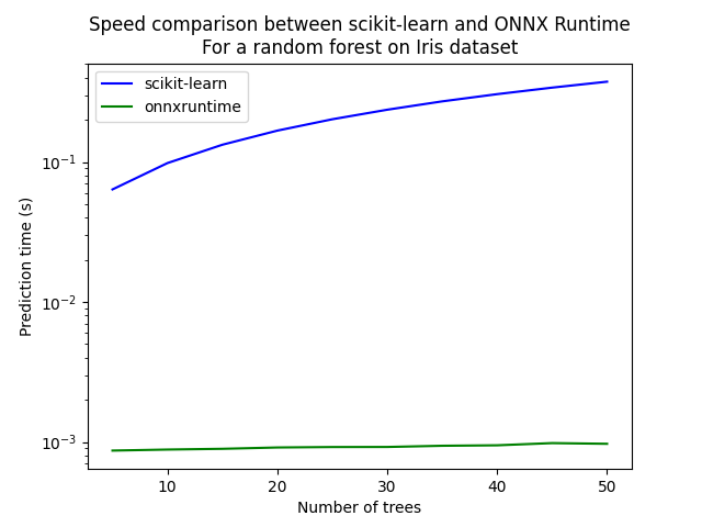
Let’s see with different number of trees.
measures = []

for n_trees in range(5, 51, 5):
    print(n_trees)
    rf = RandomForestClassifier(n_estimators=n_trees)
    rf.fit(X_train, y_train)
    initial_type = [('float_input', FloatTensorType([1, 4]))]
    onx = convert_sklearn(rf, initial_types=initial_type)
    with open("rf_iris_%d.onnx" % n_trees, "wb") as f:
        f.write(onx.SerializeToString())
    sess = rt.InferenceSession("rf_iris_%d.onnx" % n_trees, providers=rt.get_available_providers())
    def sess_predict_proba_loop(x):
        return sess.run([prob_name], {input_name: x.astype(numpy.float32)})[0]
    tsk = speed("loop(X_test, rf.predict_proba, 100)", number=5, repeat=5)
    trt = speed("loop(X_test, sess_predict_proba_loop, 100)", number=5, repeat=5)
    measures.append({'n_trees': n_trees, 'sklearn': tsk, 'rt': trt})

from pandas import DataFrame
df = DataFrame(measures)
ax = df.plot(x="n_trees", y="sklearn", label="scikit-learn", c="blue", logy=True)
df.plot(x="n_trees", y="rt", label="onnxruntime",
                ax=ax, c="green", logy=True)
ax.set_xlabel("Number of trees")
ax.set_ylabel("Prediction time (s)")
ax.set_title("Speed comparison between scikit-learn and ONNX Runtime\nFor a random forest on Iris dataset")
ax.legend()
Out:
5
Average 0.0637 min=0.0636 max=0.0639
Average 0.000869 min=0.000857 max=0.000899
10
Average 0.0982 min=0.098 max=0.0987
Average 0.000884 min=0.000873 max=0.00091
15
Average 0.133 min=0.133 max=0.133
Average 0.000895 min=0.000885 max=0.000921
20
Average 0.168 min=0.167 max=0.168
Average 0.000915 min=0.000907 max=0.00094
25
Average 0.202 min=0.201 max=0.203
Average 0.000921 min=0.000913 max=0.000948
30
Average 0.236 min=0.236 max=0.237
Average 0.000922 min=0.000914 max=0.000948
35
Average 0.271 min=0.271 max=0.271
Average 0.000941 min=0.000928 max=0.000967
40
Average 0.305 min=0.305 max=0.305
Average 0.000948 min=0.000934 max=0.000977
45
Average 0.34 min=0.339 max=0.34
Average 0.000983 min=0.000972 max=0.00101
50
Average 0.375 min=0.374 max=0.375
Average 0.000972 min=0.000966 max=0.000992

<matplotlib.legend.Legend object at 0x7feaf2025c10>
Total running time of the script: ( 3 minutes 22.159 seconds)